Usage and examples
In these tutorials we will see how data can be broken down into pieces and persistent homology can still be computed through the Mayer-Vietoris procedure. Check the notebooks if you prefer to work through these.
Torus
We compute persistent homology through two methods. First we compute persistent homology using the standard method. Then we compute this again using the Persistence Mayer Vietoris spectral sequence. At the end we compare both results and confirm that they coincide.
First we do all the relevant imports for this example
>>> import scipy.spatial.distance as dist
>>> from permaviss.sample_point_clouds.examples import torus3D, take_sample
>>> from permaviss.simplicial_complexes.vietoris_rips import vietoris_rips
>>> from permaviss.simplicial_complexes.differentials import complex_differentials
>>> from permaviss.spectral_sequence.MV_spectral_seq import create_MV_ss
We start by taking a sample of 1300 points from a torus of section radius 1 and radius from centre to section centre 3. Since this sample is too big, we take a subsample of 150 points by using a minmax method. We store it in point_cloud.
>>> X = torus_3D(1300,3)
>>> point_cloud = take_sample(X,150)
Next we compute the distance matrix of point_cloud. Also we compute the Vietoris Rips complex of point_cloud up to a maximum dimension 3 and maximum filtration radius 1.6.
>>> Dist = dist.squareform(dist.pdist(point_cloud))
>>> max_r = 1.6
>>> max_dim = 3
>>> C, R = vietoris_rips(Dist, max_r, max_dim)
Afterwards, we compute the complex differentials using arithmetic mod p, a prime number. Then we get the persistent homology of point_cloud with the specified parameters. We store the result in PerHom. Additionally, we inspect the second persistent homology group barcodes (notice that these might be empty).
>>> p = 5
>>> Diff = complex_differentials(C, p)
>>> PerHom, _, _ = persistent_homology(Diff, R, max_r, p)
>>> print(PerHom[2].barcode)
[[ 1.36770353  1.38090695]
 [ 1.51515438  1.6       ]]
Now we will proceed to compute again persistent homology of point_cloud using the Persistence Mayer-Vietoris spectral sequence instead. For this task we take the same parameters max_r, max_dim and p as before. We set max_div, which is the number of divisions along the coordinate with greater range in point_cloud, to be 2. This will indicate create_MV_ss to cover point_cloud by 8 hypercubes. Also, we set the overlap between neighbouring regions to be slightly greater than max_r. The method create_MV_ss prints the ranks of the computed pages and returns a spectral sequence object which we store in MV_ss.
>>> max_div = 2
>>> overlap = max_r*1.01
>>> MV_ss = create_MV_ss(point_cloud, max_r, max_dim, max_div, overlap, p)
PAGE: 1
[[  1   0   0   0   0   0   0   0   0]
 [ 98  14   0   0   0   0   0   0   0]
 [217  56   0   0   0   0   0   0   0]]
PAGE: 2
[[  1   0   0   0   0   0   0   0   0]
 [ 84   1   0   0   0   0   0   0   0]
 [161   5   0   0   0   0   0   0   0]]
PAGE: 3
[[  1   0   0   0   0   0   0   0   0]
 [ 84   1   0   0   0   0   0   0   0]
 [161   5   0   0   0   0   0   0   0]]
PAGE: 4
[[  1   0   0   0   0   0   0   0   0]
 [ 84   1   0   0   0   0   0   0   0]
 [161   5   0   0   0   0   0   0   0]]
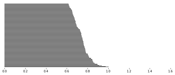
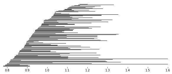
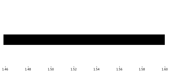
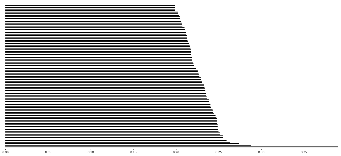
Now, we compare the computed persistent homology barcodes by both methods. Unless an AssertError comes up, this means that the computed barcodes coincide. Also, we plot the relevant barcodes.
>>> for it, PH in enumerate(MV_ss.persistent_homology):
>>>     # Check that computed barcodes coincide
>>>     assert np.array_equal(PH.barcode, PerHom[it].barcode)
>>>     # Set plotting parameters
>>>     min_r = min(PH.barcode[:,0])
>>>     step = max_r/PH.dim
>>>     width = step / 2.
>>>     fig, ax = plt.subplots(figsize = (10,4))
>>>     ax = plt.axes(frameon=False)
>>>     y_coord = 0
>>>     # Plot barcodes
>>>     for k, b in enumerate(PH.barcode):
>>>         ax.fill([b[0],b[1],b[1],b[0]],[y_coord,y_coord,y_coord+width,y_coord+width],'black',label='H0')
>>>         y_coord += step
>>>
>>>
>>>     # Show figure
>>>     ax.axes.get_yaxis().set_visible(False)
>>>     ax.set_xlim([min_r,max_r])
>>>     ax.set_ylim([-step, max_r + step])
>>>     plt.savefig("barcode_r{}.png".format(it))
>>>     plt.show()
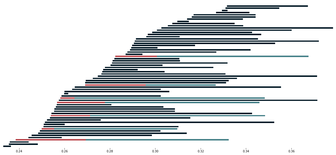
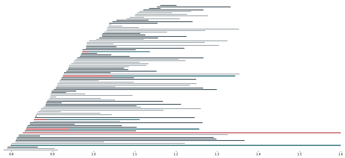
Here we look at the extension information on one dimensional persistence classes. For this we exploit the extra information stored in MV_ss. What we do is plot the one dimensional barcodes, highlighting those bars from the (0,1) position in the infinity page in red. Also, we highlight in blue when these bars are extended by a bar in the (1,0) position on the infinity page. All the black bars are only coming from classes in the (1,0) position on the infinity page.
>>> PH = MV_ss.persistent_homology
>>> start_rad = min(PH[1].barcode[:,0])
>>> end_rad = max(PH[1].barcode[:,1])
>>> persistence = end_rad - start_rad
>>> fig, ax = plt.subplots(figsize = (20,9))
>>> ax = plt.axes(frameon=False)
>>> # ax = plt.axes()
>>> step = (persistence /2) / PH[1].dim
>>> width = (step/6.)
>>> y_coord = 0
>>> for b in PH[1].barcode:
>>>     if b[0] not in MV_ss.Hom[2][1][0].barcode[:,0]:
>>>         ax.fill([b[0],b[1],b[1],b[0]],[y_coord,y_coord,y_coord+width,y_coord+width],c="#031926", edgecolor='none')
>>>     else:
>>>         index = np.argmax(b[0] <= MV_ss.Hom[2][1][0].barcode[:,0])
>>>         midpoint = MV_ss.Hom[2][1][0].barcode[index,1]
>>>         ax.fill([b[0], midpoint, midpoint, b[0]],[y_coord,y_coord,y_coord+step,y_coord+step],c="#bc4b51", edgecolor='none')
>>>         ax.fill([midpoint, b[1], b[1], midpoint],[y_coord,y_coord,y_coord+step,y_coord+step],c='#468189', edgecolor='none')
>>>         y_coord = y_coord + step
>>>
>>>     y_coord += 2 * step
>>>
>>> # Show figure
>>> ax.axes.get_yaxis().set_visible(False)
>>> ax.set_xlim([start_rad,end_rad])
>>> ax.set_ylim([-step, y_coord + step])
>>> plt.show()
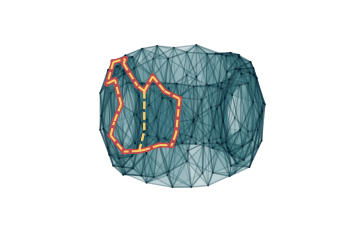
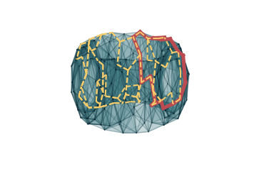
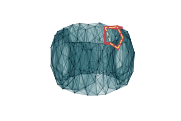
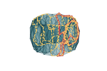
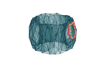
We can also study the representatives associated to these barcodes. In the following, we go through
all possible extended bars. In red, we plot representatives of a class from (1,0). These are
extended to representatives from (0,1) that we plot in dashed yellow lines.
>>> extension_indices = [i for i, x in enumerate(
>>>     np.any(MV_ss.extensions[1][0][1], axis=0)) if x]
>>>
>>> for idx_cycle in extension_indices:
>>>     # initialize plot
>>>     fig = plt.figure()
>>>     ax = fig.add_subplot(111, projection='3d')
>>>     # plot simplicial complex
>>>     # plot edges
>>>     for edge in C[1]:
>>>         start_point = point_cloud[edge[0]]
>>>         end_point = point_cloud[edge[1]]
>>>         ax.plot([start_point[0], end_point[0]],
>>>                 [start_point[1], end_point[1]],
>>>                 [start_point[2], end_point[2]],
>>>                 color="#031926",
>>>                 alpha=0.5*((max_r-Dist[edge[0],edge[1]])/max_r))
>>>
>>>     # plot vertices
>>>     poly3d = []
>>>     for face in C[2]:
>>>         triangles = []
>>>         for pt in face:
>>>             triangles.append(point_cloud[pt])
>>>
>>>         poly3d.append(triangles)
>>>
>>>     ax.add_collection3d(Poly3DCollection(poly3d, linewidths=1,
>>>                                          alpha=0.1, color='#468189'))
>>>     # plot red cycle, that is, a cycle in (1,0)
>>>     cycle = MV_ss.tot_complex_reps[1][0][1][idx_cycle]
>>>     for cover_idx in iter(cycle):
>>>         if len(cycle[cover_idx]) > 0 and np.any(cycle[cover_idx]):
>>>             for l in np.nonzero(cycle[cover_idx])[0]:
>>>                 start_pt = MV_ss.nerve_point_cloud[0][cover_idx][
>>>                     MV_ss.subcomplexes[0][cover_idx][1][int(l)][0]]
>>>                 end_pt = MV_ss.nerve_point_cloud[0][cover_idx][
>>>                     MV_ss.subcomplexes[0][cover_idx][1][int(l)][1]]
>>>                 plt.plot(
>>>                     [start_pt[0], end_pt[0]], [start_pt[1],end_pt[1]],
>>>                     [start_pt[2], end_pt[2]], c="#bc4b51", linewidth=5)
>>>         # end if
>>>     # end for
>>>     # Plot yellow cycles from (0,1) that extend the red cycle
>>>     for idx, cycle in enumerate(MV_ss.tot_complex_reps[0][1][0]):
>>>         # if it extends the cycle in (1,0)
>>>         if MV_ss.extensions[1][0][1][idx, idx_cycle] != 0:
>>>             for cover_idx in iter(cycle):
>>>                 if len(cycle[cover_idx]) > 0 and np.any(
>>>                         cycle[cover_idx]):
>>>                     for l in np.nonzero(cycle[cover_idx])[0]:
>>>                         start_pt = MV_ss.nerve_point_cloud[0][
>>>                             cover_idx][MV_ss.subcomplexes[0][
>>>                                 cover_idx][1][int(l)][0]]
>>>                         end_pt = MV_ss.nerve_point_cloud[0][cover_idx][
>>>                             MV_ss.subcomplexes[0][cover_idx][
>>>                                 1][int(l)][1]]
>>>                         plt.plot([start_pt[0], end_pt[0]],
>>>                                  [start_pt[1],end_pt[1]],
>>>                                  [start_pt[2], end_pt[2]],
>>>                                  '--', c='#f7cd6c', linewidth=2)
>>>                 # end if
>>>             # end for
>>>         # end if
>>>     # end for
>>>     # Then we show the figure
>>>     ax.grid(False)
>>>     ax.set_axis_off()
>>>     plt.show()
>>>     plt.close(fig)
Random 3D point cloud
We can repeat the same procedure as with the torus, but with random 3D point clouds. First we do all the relevant imports for this example
>>> import scipy.spatial.distance as dist
>>> from permaviss.sample_point_clouds.examples import random_cube, take_sample
>>> from permaviss.simplicial_complexes.vietoris_rips import vietoris_rips
>>> from permaviss.simplicial_complexes.differentials import complex_differentials
>>> from permaviss.spectral_sequence.MV_spectral_seq import create_MV_ss
We start by taking a sample of 1300 points from a torus of section radius 1 and radius from center to section center 3. Since this sample is too big, we take a subsample of 91 points by using a minmax method. We store it in point_cloud.
>>> X = random_cube(1300,3)
>>> point_cloud = take_sample(X,91)
Next we compute the distance matrix of point_cloud. Also we compute the Vietoris Rips complex of point_cloud up to a maximum dimension 3 and maximum filtration radius 1.6.
>>> Dist = dist.squareform(dist.pdist(point_cloud))
>>> max_r = 0.39
>>> max_dim = 4
>>> C, R = vietoris_rips(Dist, max_r, max_dim)
Afterwards, we compute the complex differentials using arithmetic mod p, a prime number. Then we get the persistent homology of point_cloud with the specified parameters. We store the result in PerHom.
>>> p = 5
>>> Diff = complex_differentials(C, p)
>>> PerHom, _, _ = persistent_homology(Diff, R, max_r, p)
Now we will proceed to compute again persistent homology of point_cloud using the Persistence Mayer-Vietoris spectral sequence instead. For this task we take the same parameters max_r, max_dim and p as before. We set max_div, which is the number of divisions along the coordinate with greater range in point_cloud, to be 2. This will indicate create_MV_ss to cover point_cloud by 8 hypercubes. Also, we set the overlap between neighbouring regions to be slightly greater than max_r. The method create_MV_ss prints the ranks of the computed pages and returns a spectral sequence object which we store in MV_ss.
>>> max_div = 2
>>> overlap = max_r*1.01
>>> MV_ss = create_MV_ss(point_cloud, max_r, max_dim, max_div, overlap, p)
    PAGE: 1
    [[  0   0   0   0   0   0   0   0   0]
     [ 11   1   0   0   0   0   0   0   0]
     [ 91  25   0   0   0   0   0   0   0]
     [208 231 236 227 168  84  24   3   0]]
    PAGE: 2
    [[ 0  0  0  0  0  0  0  0  0]
     [10  0  0  0  0  0  0  0  0]
     [67  3  0  0  0  0  0  0  0]
     [91  7  2  0  0  0  0  0  0]]
    PAGE: 3
    [[ 0  0  0  0  0  0  0  0  0]
     [10  0  0  0  0  0  0  0  0]
     [65  3  0  0  0  0  0  0  0]
     [91  7  1  0  0  0  0  0  0]]
    PAGE: 4
    [[ 0  0  0  0  0  0  0  0  0]
     [10  0  0  0  0  0  0  0  0]
     [65  3  0  0  0  0  0  0  0]
     [91  7  1  0  0  0  0  0  0]]
    PAGE: 5
    [[ 0  0  0  0  0  0  0  0  0]
     [10  0  0  0  0  0  0  0  0]
     [65  3  0  0  0  0  0  0  0]
     [91  7  1  0  0  0  0  0  0]]
In particular, notice that in this example the second page differential is nonzero. Now, we compare the computed persistent homology barcodes by both methods. Unless an AssertError comes up, this means that the computed barcodes coincide. Also, we plot the relevant barcodes.
>>> for it, PH in enumerate(MV_ss.persistent_homology):
>>>     # Check that computed barcodes coincide
>>>     assert np.array_equal(PH.barcode, PerHom[it].barcode)
>>>     # Set plotting parameters
>>>     min_r = min(PH.barcode[:,0])
>>>     step = max_r/PH.dim
>>>     width = step / 2.
>>>     fig, ax = plt.subplots(figsize = (10,4))
>>>     ax = plt.axes(frameon=False)
>>>     y_coord = 0
>>>     # Plot barcodes
>>>     for k, b in enumerate(PH.barcode):
>>>         ax.fill([b[0],b[1],b[1],b[0]],[y_coord,y_coord,y_coord+width,y_coord+width],'black',label='H0')
>>>         y_coord += step
>>>
>>>
>>>     # Show figure
>>>     ax.axes.get_yaxis().set_visible(False)
>>>     ax.set_xlim([min_r,max_r])
>>>     ax.set_ylim([-step, max_r + step])
>>>     plt.savefig("barcode_r{}.png".format(it))
>>>     plt.show()

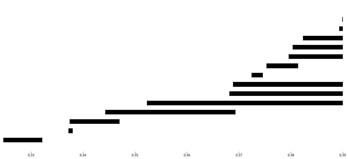
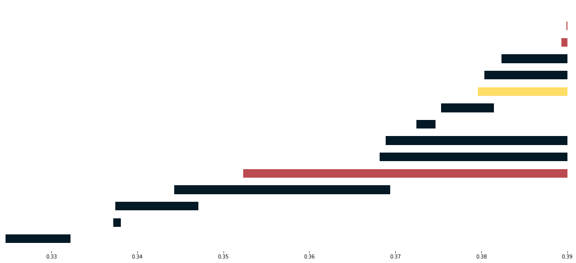
Here we look at the extension information on one dimensional persistence classes. For this we exploit the extra information stored in MV_ss. What we do is plot the one dimensional barcodes, highlighting those bars from the (0,1) position in the infinity page in red. Also, we highlight in blue when these bars are extended by a bar in the (1,0) position on the infinity page. All the black bars are only coming from classes in the (1,0) position on the infinity page. Similarly, we also highlight the bars on the second diagonal positions (2,0), (1,1), (0,2) by colours yellow, read and blue respectively. If a bar is not extended we write it in black (bars which are not extended are completely contained in (0,2)
>>> PH = MV_ss.persistent_homology
>>> no_diag = 3
>>> colors = [ "#ffdd66", "#bc4b51", "#468189"]
>>> for diag in range(1, no_diag):
>>>     start_rad = min(PH[diag].barcode[:,0])
>>>     end_rad = max(PH[diag].barcode[:,1])
>>>     persistence = end_rad - start_rad
>>>     fig, ax = plt.subplots(figsize = (20,9))
>>>     ax = plt.axes(frameon=False)
>>>     # ax = plt.axes()
>>>     step = (persistence /2) / PH[diag].dim
>>>     width = (step/6.)
>>>     y_coord = 0
>>>     for b in PH[diag].barcode:
>>>         current_rad = b[0]
>>>         for k in range(diag + 1):
>>>             if k == diag and current_rad == b[0]:
>>>                 break
>>>             if len(MV_ss.Hom[MV_ss.no_pages - 1][diag - k][k].barcode) != 0:
>>>                 for i, rad in enumerate(MV_ss.Hom[
>>>                         MV_ss.no_pages - 1][diag - k][k].barcode[:,0]):
>>>                     if np.allclose(rad, current_rad):
>>>                         next_rad = MV_ss.Hom[
>>>                             MV_ss.no_pages - 1][diag - k][k].barcode[i,1]
>>>                         ax.fill([current_rad, next_rad, next_rad, current_rad],
>>>                                 [y_coord,y_coord,y_coord+step,y_coord+step],
>>>                                 c=colors[k + no_diag - diag - 1])
>>>                         current_rad = next_rad
>>>                     # end if
>>>                 # end for
>>>             # end if
>>>
>>>         # end for
>>>         if current_rad < b[1]:
>>>             ax.fill([current_rad, b[1], b[1], current_rad],
>>>                             [y_coord,y_coord,y_coord+step,y_coord+step],
>>>                             c="#031926")
>>>         # end if
>>>         y_coord = y_coord + 2 * step
>>>     # end for
>>>
>>>     # Show figure
>>>     ax.axes.get_yaxis().set_visible(False)
>>>     ax.set_xlim([start_rad, end_rad])
>>>     ax.set_ylim([-step, y_coord + step])
>>>     plt.show()